Setting up a custom model¶

In principle, any custom model can be used in ALPro. This tutorial allows shows how to set up a model with any given profile of magnetic field and density without using ALPro’s inbuilt models.

[1]:

%matplotlib inline
import matplotlib.pyplot as plt
import numpy as np
import alpro
alpro.util.set_default_plot_params()

[2]:

s = alpro.Survival("custom")

Warning: Custom model specified - make sure get_B & density methods are populated or domain set manually!

There are two ways to set up a custom model. Minimally, ALPRO needs a domain instance initialised, and then the following variables need to be initialised:

ne: the electron density
B: the perpendicular magnetic field
phi: the angle the magnetic field vector makes with the \(y\) axis
deltaL: the size of each domain

So one can easily just specify these manually. As an example, let’s set up a perpendicular field that varies randomly and makes a random angle with the \(y\)-axis. We’ll give a characteristic field strength of \(10\, \mu {\rm G}\) and typical cell sizes of kpc.

[3]:

np.random.seed(42)
s.initialise_domain()
s.domain.ne = np.random.random(size=10) * 0.01
s.domain.B = np.random.random(size=10) * 1e-5
s.domain.deltaL = np.random.random(size=10) * 10.0
redge = np.cumsum(s.domain.deltaL)
s.domain.phi = np.random.random(size=10) * 2.0 * np.pi
_ = plt.step(redge, s.domain.B, where="pre")

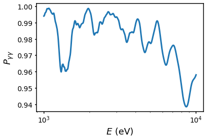
We can then compute the survival probability

[4]:

energies = np.logspace(3,4,100)
s.set_params(g = 1e-12 * 1e-9, mass = 1e-11)
s.propagate(energies=energies, pol="y")
fig = s.default_plot(mode="survival")

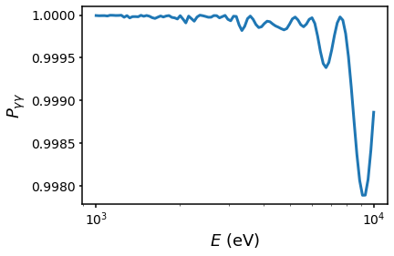
Alternatively, you may want to set up a cell-based model with a given density and magnetic field strength with radius, then initialise a random cell model. In this case we’re just going to use some arbitrary functions, but you could use, for example, power-law profiles or a universal pressure profile to set these up.

[38]:

def get_B(r):
    return (1e-5 * (r/25.0)**-0.5)

def get_ne(r):
    return (0.1 * (r/25.0)**-2)

# this controls the size of each random cell. Normally chosen using a power-law, but you can use
# any function or supply a float for a constant cell size
def coherence():
    return (np.random.random() * 10.0)

s = alpro.Survival("custom")      # initialise model

# set up get_B and density methods
s.cluster.get_B = get_B
s.cluster.density = get_ne

# initialise domain subclass using this profile
s.initialise_domain(s.cluster.profile)

# create a random cell model
s.domain.create_box_array(500.0, 1, coherence = coherence)

# plot the model
_ = plt.step(s.domain.r, s.domain.Bx, where="pre")
_ = plt.step(s.domain.r, s.domain.By, where="pre")

Warning: Custom model specified - make sure get_B & density methods are populated or domain set manually!

[39]:

energies = np.logspace(3,4,1000)
s.set_params(g = 1e-12 * 1e-9, mass = 1e-13)
s.propagate(energies=energies, pol="both")
fig = s.default_plot(mode="survival")