Tests of the code¶

This notebook is designed to document some simple tests of the photon-ALP propagation code ALPro. Most of these tests can be run by running

python -m unittest alpro.test

from the command line.

[1]:

%matplotlib inline
import alpro
import matplotlib.pyplot as plt
alpro.util.set_default_plot_params()

1. Single Domain Test¶

First, let’s compare an idealised pure polarization state solution to the analytic solution given by

\[ \begin{align}\begin{aligned} P_{\gamma \rightarrow a} = \frac{\Theta^2}{1+\Theta^2} \sin^2 (\Delta_{\rm eff} \sqrt{1+\Theta^2} L),\\where\end{aligned}\end{align} \]

\[ \begin{align}\begin{aligned} \Theta=2B_\perp E g_{a \gamma}/m_{\rm eff}^2\\and\end{aligned}\end{align} \]

\[ \begin{align}\begin{aligned} \Delta_{\rm eff}=m_{\rm eff}^2 L / (4E)\\where :math:`m_{\rm eff}^2=m_a^2-\omega_{\rm pl}^2`.\end{aligned}\end{align} \]

The model here is a single domain of width \(10~{\rm kpc}\), with uniform field \(B=10 \mu{\rm G}\) oriented along the \(y\)-axis. The polarization state is \((0,1,0)\) and we use energies from \(1-10~{\rm keV}\).

This test also checks for agreement within a relative tolerance of \(10^{-6}\) between the theoretical and numerical calculations.

[2]:

test = alpro.test.RunTest()
test.test_analytic(subplot=111)

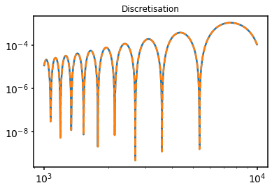
2. Discretisation Test¶

In our second test, we repeat the above test, but now compare a single domain to a discretised uniform field. Specifically the result from 1 uniform cell of size \(L\) to \(10\) uniform cells of size \(L/10\). This should give an identical result. The parameters and procedure are identical to our first test.

[3]:

test.test_discretise(subplot=111)

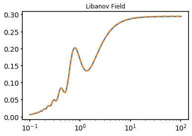
3. Libanov field model v Marsh¶

This tests a uniform field model from Libanov & Troitsky (2021), which is originally described by Gourgouliatos et al. (2010), against M. C. David Marsh’s code. This test uses a large scale uniform field and energies in the GeV regime. The field components are given by

\[\begin{split}B_r = \frac{2 \cos\theta}{r^2} f(r) \\ B_\theta = - \frac{\sin \theta}{r} f'(r) \\ B_\phi = \frac{\alpha \sin \theta}{r} f(r) \, ,\end{split}\]

where \(\alpha\) solves a transcendental equation and is approximately given by \(\alpha= 5.76\). The function \(f(r)\) is given by

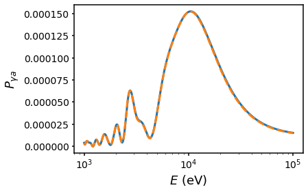
\[f(r) =c_1\Big( \alpha \cos (\alpha u) - \frac{\sin(\alpha u)}{u} - u^2\left( \alpha \cos\alpha - \sin \alpha \right) \Big) \, .\]

The form of the field is plotted below, before we plot the ALP result. Note that this is now the survival probability on a linear axis. We find cosmetically perfect agreement between our results and Marsh. the Libanov results are smoothed with the Fermi response which is presumably the reason for the difference, but the overall form is similar.

[4]:

test.test_marsh(subplot=111)

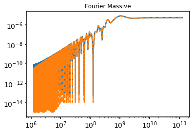
4. Massive Fourier Formalism¶

[5]:

test.test_fourier_massive(subplot=111)

/Users/matthews/Library/Python/3.7/lib/python/site-packages/alpro/test.py:153: RuntimeWarning: invalid value encountered in greater
  select = (P1 > 1e-7)

5. Massless Fourier Formalism¶

[6]:

test.test_fourier_massless(subplot=111)

6. Domain Field Test v Analytic¶

This tests a cell-based domain model against an analytic solution computed by Pierluca Carenza.

[7]:

import numpy as np
def setup_carenza_model():
    s = alpro.Survival("custom")
    s.init_model()
    r, f = np.genfromtxt("../data/Bfield_Carenza.dat", unpack=True)
    s.set_params(g=1e-12 * 1e-9, mass=1e-11)
    s.domain.deltaL = r[1:] - r[:-1]
    s.domain.r = r[:-1]
    s.domain.rcen = 0.5 * (r[1:] + r[:-1])
    s.domain.ne = np.zeros_like(s.domain.r)
    s.domain.Bx = f[:-1] * 1e-6
    s.domain.By = np.zeros_like (s.domain.Bx)
    s.domain.B = np.sqrt(s.domain.Bx**2  + s.domain.By **2)
    s.domain.phi = np.arctan2(s.domain.Bx,s.domain.By)
    return (s)

energies,P = np.genfromtxt("../data/Prob_Carenza.dat", unpack=True)

s = setup_carenza_model()
Pcode, _ = s.propagate(s.domain, energies, pol="x")

# make the default plot and overplot Pierluca's solution
s.default_plot()
plt.plot(energies, P, c="C1", ls="--", label="Carenza analytic")

Warning: Custom model specified - make sure get_B & density methods are populated or domain set manually!

[7]:

[<matplotlib.lines.Line2D at 0x13763a890>]

Additional Tests¶

I’ve done a number of other tests - using the code in various regimes in terms of density, energy, magnetic field strength. I’ve also tested alpro against gammaALPs, with near identical results in the X-ray regime, but these are not documented here for the moment.

Tests of the code

Contents